Hypoplastic Clay
Hypoplastic clay is applicable for the modeling of soft fine grain soils. Similarly to all other models it belongs to the family of standard phenomenological models. As for the description of the soil response it falls into the group of critical state models (Cam clay, Generalized cam clay). This model, however, accounts for the nonlinear response of soils both in load and unloading. In comparison to other models based on the theory of plasticity, it allows for the calculation of total strains only. It thus makes no difference between elastic and plastic strains. Indication of type and location of a potential failure, in other models provided by the plot of equivalent deviatoric plastic strain, can be in case of hypoplastic clay represented by the distribution of the mobilized angle of internal friction.
When describing the soil response, the model allows for reflecting a different stiffness in loading and unloading, softening or hardening in dependence on the soil compaction and the change of volume in shearing (dilation, compression). The current stiffness depends on only the load direction, but also on the current state of soil given by its porosity. Unlike Cam clay models, it strictly excludes tensile stresses in soil, see Figure 1a.
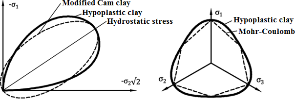 Figure 1: State boundary of hypoplastic model - (a) comparison with the yield surface of Cam clay model in the meridial plane, (b) comparison with the yield surface of Mohr-Coulomb model in the deviatoric plane
In case of hypoplastic model the standard yield surface is replaced by so called Boundary state surface. Its projection into the deviatoric plane is similar to the model, see Figure 1b. The flow rule is non-associated resulting into a nonsymmetric stiffness matrix (compare e.g. with the Mohr-Coulomb model when having different values for the angle of internal friction φ and the dilation angle ψ). Details regarding the model formulation can be found in [1].
Model parameters
The basic variant of the model requires inputting five material parameters:
- Angle of internal friction for constant volume (critical angle of internal friction) φcv
- Slope of swelling line κ*
- Slope of normal consolidation line (NCL - normal consolidation line) λ*
- Origin of the normal consolidation line N
- Ratio of unit and shear modulus r
Parameters κ*, λ* and N determine a bilinear diagram of isotropic consolidation in a log-log scale, Figure 2a. Providing the parameters of the bilinear Cam clay model (in semi-logarithmic scale, Figure 2b) are available, it is possible to input these values and the parameters of the hypoplastic model are back calculated. Parameters of the bilinear Cam clay model are:
- Slope of swelling line κ (in semi-logarithmic scale)
- Slope of normal consolidation line λ (in semi-logarithmic scale)
- Void ratio emax for normal isotropic consolidation by pressure of 1kPa
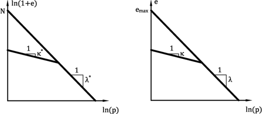 Figure 2:Bilinear diagram of isotropic consolidation - (a) Hypoplastic clay, (b) Cam clay model
Critical angle of internal friction φcv
- Identical for both original (undisturbed) and reconstituted subsequently consolidated sample
- Can be determined from standard triaxial test applying different cell pressures on a reconstituted sample
- Both drained and undrained (faster) test can be performed
- Most common values are in range of 18° - 35°
Slope of normal consolidation line λ*
- It is determined graphically from the loading branch of oedometric or isotropic consolidation test, see Figure 3
- For stiff clays it is preferable to run the test on a reconstituted sample
- Most common values are in range of 0.04 - 0.15
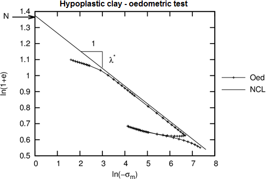 Figure. 3: Simulation of oedometric test with hypoplastic model
Slope of swelling line κ*
- It can be determined similarly as parameter λ* graphically or by performing a parametric study - comparing measurements and simulation along the unloading branch of oedometric or isotropic consolidation test, see Figure 3
- Most common values κ are in range of 0.01 - 0.02
- Ratio λ/κ should be large than 4.0
Origin of normal consolidation line N
- It is determined graphically from the loading branch of oedometric or isotropic consolidation test
- The test should be performed on an undisturbed sample - when searching for the intersection lambda line with the vertical axis it is possible to determine the slope lambda obtained from a reconstituted sample, see Figure 3
- Most common values are in range 0.8 - 1.6
Ratio of unit and shear modulus r
- The physical meaning of this parameter is given by the expression r = Ki/Gi
- Ki corresponds to the tangent unit modulus from isotropic compression according to the normal consolidation line
- Gi corresponds to the tangent shear modulus for undrained shear test assuming the same stress state
- Parameter r can be determined by a parametric study of shear triaxial test
- Most common values are in range 0.05 - 0.7
Setting initial state of soil
In hypoplastic clay the current state of soil is associated with the current compaction represented by the void ratio. Model implementation allows for inputting the initial or current void ratio either directly or it can be back calculated using the input preconsolidation pressure OCR. In the first case, the input value e0 corresponds to the void ratio measured on an unloaded sample extracted from a given depth. In the second case, the inputted value of ecurr corresponds to the void ratio of a stressed soil. In the last case, the value of OCR is specified. This parameter represents the ratio between the mean stress on NCL and the initial mean stress, see Figure 4b.
When initializing the task using the Ko procedure, the initial stress state at the beginning of the second stage is assigned the current stress state. If adopting standard analysis in the first stage (the hypoplastic clay model is introduced already in the first calculation stage) where the soil is loaded by its self-weight, the value of initial stress pin = 1 kPa is assumed and it holds ecurr = e0. Providing a different material (e.g., elastic material is considered in the first calculation stage) is replaced by the hypoplastic clay model, the initial state of stress derived in the previous stage is adopted. Recall that when using elastic material in the first calculation stage the resulting stress state corresponds to the results provided by Ko procedure for Ko (ν is the Poisson's ratio).
![]()
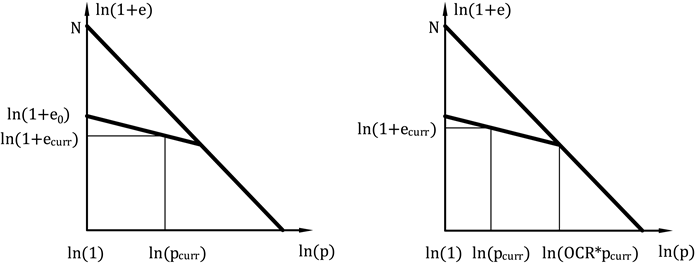 Figure 4: Initiation of void ratio - (a) with the help of initial void ratio, (b) initiation by OCR
It is clear from Figure 5 that for normally consolidated soils the state for which OCR = 1.0 corresponds to an isotropic consolidation only, thus for Ko = 1.0. If the soil experiences a non-zero deviatoric stress state the corresponding OCR for a normally consolidated soil is greater than 1.0. An exact value of depends on both the soil parameters and stress path (the value of Ko). Figure 5 shows the dependence of the minimum for various values of Ko and different types of clayey soils. Particular values are also stored in Table 1. The basic material parameters of this set of soils are listed in Table 2.
The choice of OCR = 1.0 for normally consolidated soils with Ko not equal to 1.0 creates a non-acceptable stress state which may result in the loss of convergence.
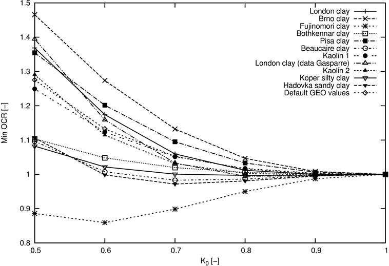 Figure 5: Dependence of OCR on the coefficient of earth pressure at rest Ko
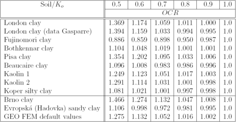 Table 1: Oveconsolidation ratio OCR of the selected soils as function of Ko value
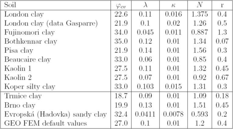 Table 2: Material parameters of the selected soils
Intergranular strain
The basic version of the model is suitable in analyses with a prevailing direction of the stress loading path. In cases with cyclic loading (loading-unloading-reloading) it is more suitable to use an advanced formulation with the concept of intergranular strain. This allows for constraining a unacceptable increase of permanent deformation arising during small repeating changes in load (ratcheting). Introducing intergranular strain allows for the modeling of large stiffness, which clays experience during small strains. This option is not part on any other models implemented in GEO FEM. The concept of intergranular strain assumes that the total soil deformation consists of a small deformation of an intergranular layer (integranular strain) and deformation caused by mutual sliding of grains. Changing the load path changes first the intergranular strain. Upon reaching the limit value of the intergranular strain, the deformation associated with the motion of grains sets on.
Adopting the concept of intergranular strain requires five additional parameters:
- Range of elastic intergranular strain R
- Parameters mR and mT control the small strain stiffness
- Parameters βr and χ control the degree of stiffness degradation with increasing shear strain
These parameters are calibrated after knowing already the material data of the basic hypoplastic model.
Margin of elastic intergranular deformation R
- It determines the range of maximal intergranular strain
- It can be determined by a parametric study of the degradation curve G = G(εs), Figure 5
- Alternatively it can be considered as material independent constant R = 10-4
- Most common values are in range 2*10-5 - 1*10-4
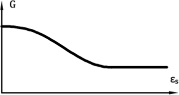 Figure 6: Curve describing the loss of stiffness of shear modulus
Parameter mR
- It determines the magnitude of the shear modulus when changing the loading path in the meridian plane (σm - J) o 180°
- Linear ratio between parameter mR and the initial shear modulus G0 is provided by G0 = p*(mr/(r* λ*)
- The initial shear modulus can be determined from the measurement of shear wave propagation [2]
- Most common values are in range 4.0 - 20.0
Parameter mT
- It determines the magnitude of the shear modulus when changing the loading path in the meridian plane (σm - J) o 90°
- It holds mR/mT = G0/G90
- The ratio of initial moduli can be estimated from the ratio of these moduli for larger strains. The value of the mR/mT ratio is commonly in the range of 1.0 - 2.0
- Most common values of mT are in range 2.0 - 20.0
Parameters βr and χ
- Determine the rate of stiffness degradation with increasing shear strain
- It can be determined by a parametric study of the degradation curve G = G(εs)
- Most common values of parameter βr are in range 0.05 - 0.5
- Most common values of parameter χ are in range 0.5 - 6
Literature:
[1] D. Mašín, A hypoplastic constitutive model for clays, International Journal for Numerical and Analytical Methods in Geomechanics., 29:311-336, 2005.